
Quick math on why different solar arrays perform differently?
The mathematical portion of the East-West and single-axis array comparison.

This article is intended to explore the mathematics that underpin the evaluation of the performance of a solar array type. We use this type of math in our East-West vs single-axis tracked array analysis.
Important concepts before we get started.
The energy available to photovoltaic systems depends on the Sun-Earth relationship and the specific location of the system on Earth’s surface. Before we start, let’s get a couple of the basics of the Earth-Sun relationship down:
The Earth’s orbit around the Sun is slightly elliptical, leading to variations in the Sun’s position in our sky by a particular hour from day to day. The equation of time corrects for this variance.
The Earth rotates on a 24-hour schedule.
The solar constant measures the power per area (solar irradiance) of sunlight as it hits Earth’s atmosphere: 1,361 Watts per square meter.
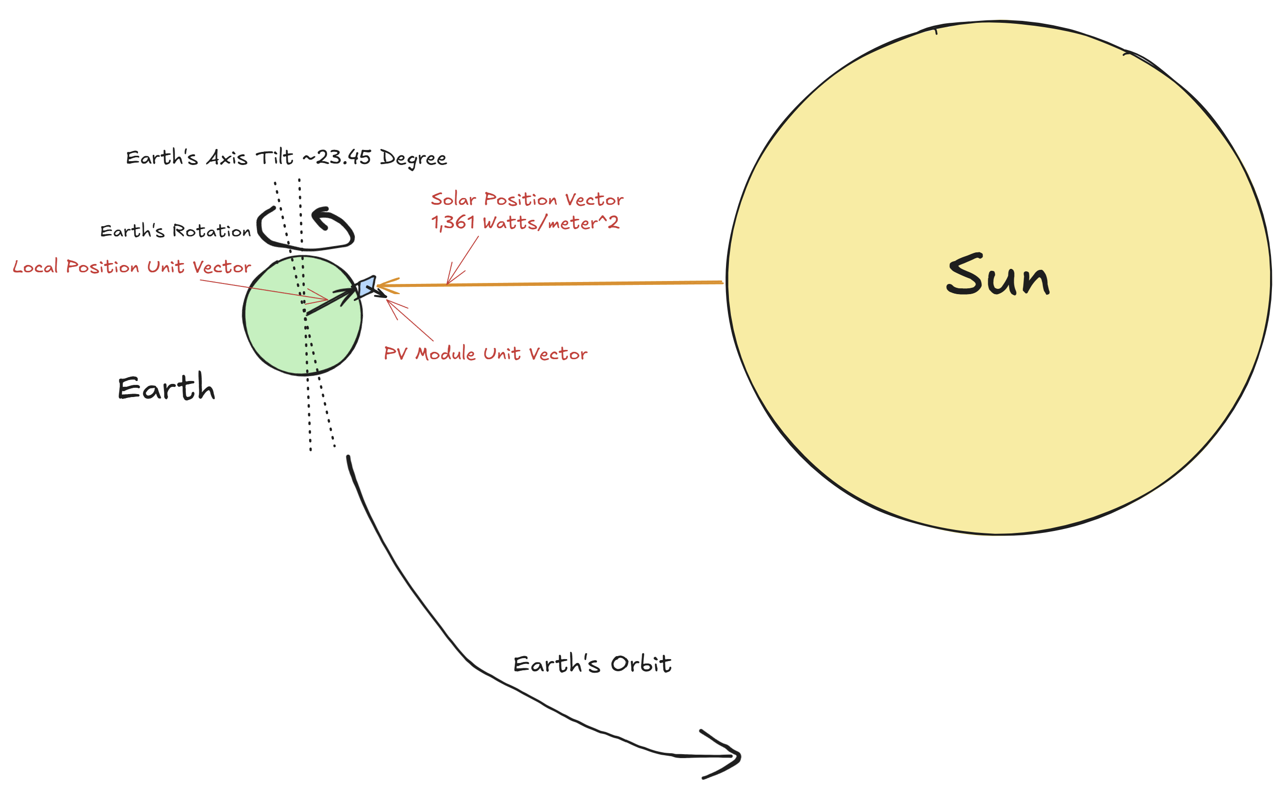
The amount of sunlight available is determined by the relationship between the local position on Earth, the orientation of the PV module, and the solar position vector, based on the relative positions of the Earth and the Sun.
The solar position vector magnitude is the solar constant, with a direction determined by the time of day and the Sun’s declination angle, determined by Earth’s axial tilt and orbit.
The local position vector extends from Earth’s center to the PV’s position on Earth’s surface, which is determined by its latitude, longitude, and elevation.
The PV module vector is based on the azimuth and module tilt.
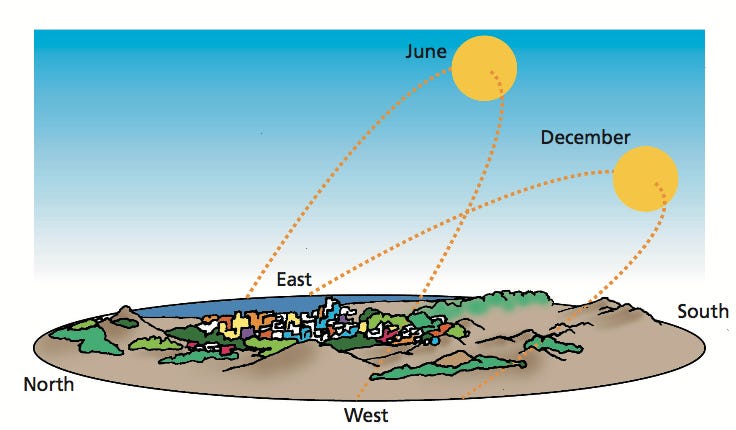
The solar position vector and local position vector affect how sunlight appears at any one spot. The latitude of the position and the declination angle determine the elevation and duration during which the sun appears in the sky. A shallower angle, common in winter in the Northern hemisphere, will lead to a lower elevation and a more significant percentage of Earth’s 24hr rotation with the Sun appearing below the horizon. This scenario is the exact inverse in the southern hemisphere, with increasingly lower latitudes leading to the Sun appearing increasingly more northward at a lower elevation.
First, we determine our sunlight vector.
We must simplify this relationship down to the interaction of two vectors by reasoning that both the local position vector and the solar position vector can be simplified to one sunlight vector, which contains the magnitude of solar irradiance and the direction from which it approaches our location. In order to define this vector, we must find the sun’s elevation angle— the up and down component of the Sun’s position, and its azimuth angle—the map directions component (East, West, North, South). To do so, we change our reference point to our local position with a bit of spherical geometry. We relate the sunlight vector to the zenith, our local position vector projected out to the celestial sphere, and the Earth’s North Pole to understand the solar elevation and azimuth angles.
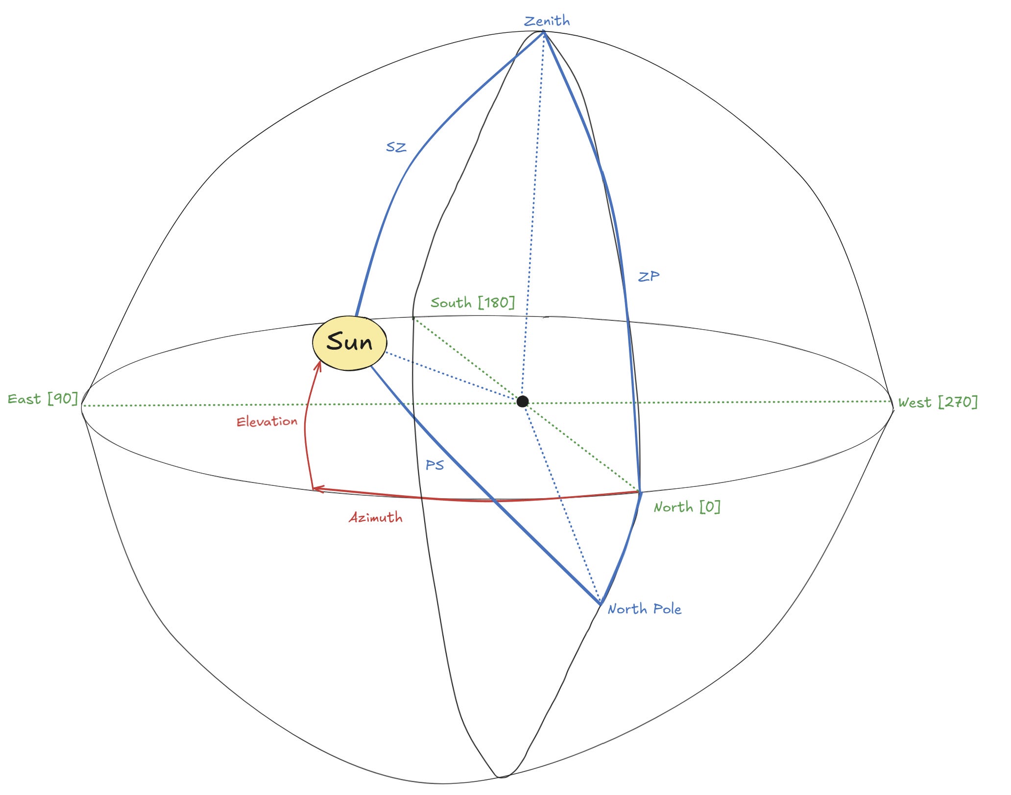
ZP is the angular distance from the zenith to the North Pole and is equal to 90 degrees - ɸ.
ɸ is the latitude of your location.
PS is the angular distance from the North Pole to the Sun and is equal to 90 degrees - δ.
δ is the declination angle of the Sun, due to Earth’s axial tilt and the day of year.
SZ is the zenith to Sun position distance, equal to 90 degrees minus the elevation.
Elevation is the vertical angle between the Sun and the horizon.
<PZS, is the azimuth angle, the angle between the North pole and the sun.
<ZPS, is the solar hour angle H, the angle between the zenith and the sun.
The vertical component, elevation α, can be solved for:
The horizontal component, azimuth A, can be solved for:
Then we substitute in the value of sin(α).
The azimuth cannot be solved for by using cosine, since it can be any of the four quadrants (NE, NW, SE, SW). For this reason, we will use the tangent of A. We find the sine of the azimuth by using the law of sines.
Then we combine these together to define the tangent of the sunlight vector’s azimuth.
The azimuth and elevation define the polar coordinates of the sunlight vector.
A note on solving for the declination angle and the solar hour angle
Declination and local solar time might be new concepts, so I’ll define how we find these values. Declination is determined by the number of days we are from a solstice, because we know the declination angle at the solstice is zero, and we can use it as a reference for other points in the year. In December, the North Pole is tilted away from the Sun by 23.45 degrees. It is the polar opposite of the June solstice.
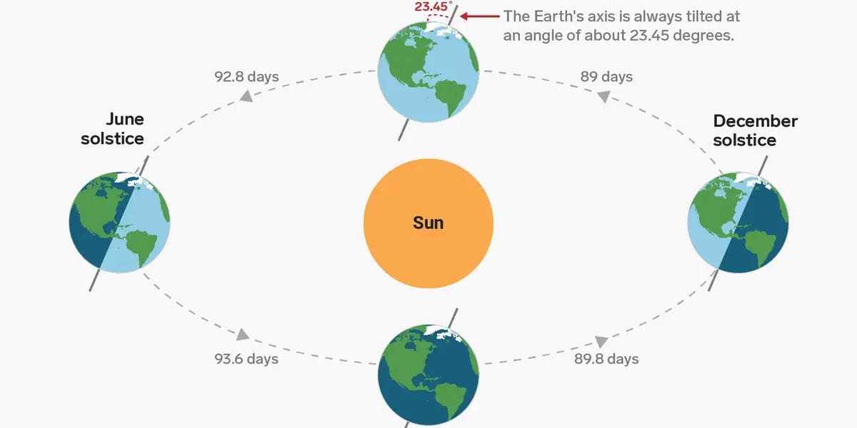
We can use the known angle of -23.45 degrees on the December solstice to define our current angle based on the N number of days from the beginning of the new year.
We could just as easily define the inclination angle from the number of days we are away from the equinoxes, which are days when the Sun’s declination is zero degrees.
The solar time is converted to your local time based on your longitude (λ) and the equation of time, a correction for Earth’s orbital eccentricity. λ(std) is the standard meridian of your local time zone.
We then convert this solar time into an hour angle (H).
Second, we determine our module position vector.
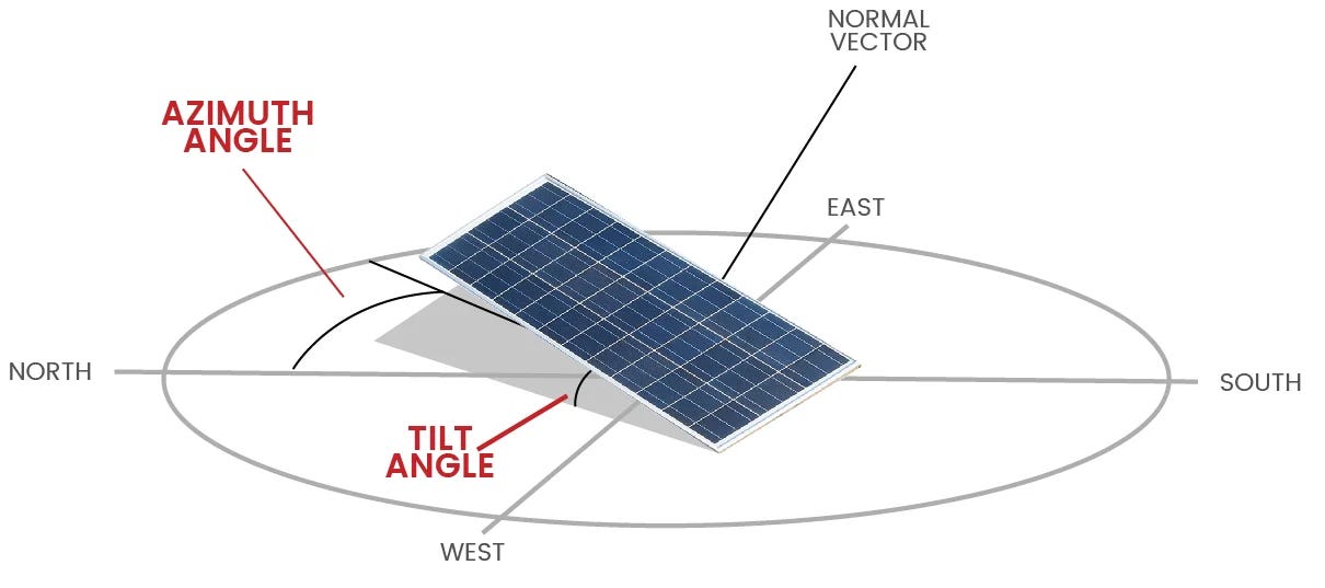
Next, we find the normal vector, N, to the PV module surface. For this, we need to know the direction the panel is facing, using spherical coordinates. We will then convert the spherical coordinates to Cartesian coordinates.
Tilt angle β: Angle between the normal vector of the PV module and your position’s zenith. This is equivalent to the angle between the horizontal plane and the panel’s front face.
Azimuth angle γ: Direction the panel faces (0° = North, 90° = East, 180° = South, 270° = West)
Third, we solve for the effective irradiance.
Then we determine how much of that light we can capture by taking the dot product between the sunlight and panel vectors to determine the amount of sunlight that can effectively enter the PV cells in the array. We then multiply this product by the solar constant to understand the effective irradiance the PV array will be exposed to
Where:
α = solar elevation angle
A = solar azimuth angle
β = panel tilt angle
γ = panel azimuth angle
Then we can plug in the sun and earth parameters into the solar elevation and azimuth.
We can interpret this equation by examining its component parts.
sin(δ)sin(φ)cos(β)
This represents the coupling between the solar declination and your position’s latitude. It will remain constant throughout changes within each day.
sin(δ)cos(φ)sin(β)cos(γ)
This models the effectiveness of the panel orientation given the Sun’s current declination and your installation’s latitude.
cos(δ)cos(H)(cos(φ)cos(β) + sin(φ)sin(β)cos(γ))
Intra-day energy fluctuation as dictated by the Sun’s position vector and the panels’ orientation. This is the dominant component in the middle of the day as the Hour component approaches zero at solar noon.
cos(δ)sin(β)sin(γ)sin(H)
The alignment between the panel’s orientation and the horizontal change in the Sun’s position over the day. This contributes to sunlight collected by the tracked and East-West arrays in the morning and afternoon. There is little expected contribution of this factor to a South or north-facing fixed-axis array.
So why do single-axis trackers collect more sunlight per panel?
We can crudely demonstrate by approximating the panel tilt of a single-axis tracker to be approximately equal to the solar hour component $\beta\approx H$. Meanwhile, we expect to see some difference between the angle of the panel and that of the Sun in the fixed East-West array.
Let’s compare the performance when we assume a location of Los Angeles, φ = 34, during an equinox, δ = 0. Around noon, the benefits are slight when compared to the morning and afternoon.
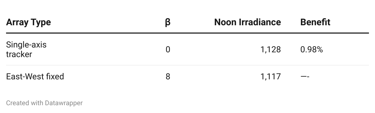
Table 1: Performance variance around noon
The advantage that the single-axis tracker has during the mornings and afternoons is quite significant, due to its ability to have a much larger tilt angle towards the rising and setting sun. This leads to a much broader power generation profile versus its fixed tilt counterpart.
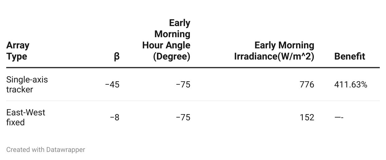
Table 2: Performance variance around the early morning
The comparisons, looking at the dominant component, indicate that the primary difference in performance between the single-axis tracker and the East-West array is the performance in the early morning or late afternoon. This advantage declines as the hours approach noon, resulting in minimal differences in power during the mid-morning and solar noon. Performance differences can be easily made up by increasing the number of panels in the East-West array to compensate for its comparative performance disadvantage.
To better understand the performance difference between these two systems, it is better to simulate rather than run simple hand calcs. To see this in action, check out my blog asking if it’s time to ditch your single-axis arrays for a simpler East-West array.